1 MCMC

Hierarchical models can get very complex quickly, creating big computational headaches. For $$\lambda (\theta |x)=\frac{p_{\theta }(x)\lambda (\theta )}{{\int }_{\mathrm{\Omega }}{p}_{\zeta }(x)\lambda (\zeta )\mathrm{d}\zeta },$$ the integral is often intractable.
A computational strategy is to set up a Markov chain with stationary distribution ${\displaystyle \propto p_{\theta }(x)\lambda (\theta )}$, and run it to get approximate samples from ${\displaystyle \lambda (\theta |x)}$.

Compared with Markov chain in probability, the notation here is more Bayesian.

The marginal distribution of ${\displaystyle X^{(1)}}$ is $${\pi }_1(y)=\mathbb{P}(X^{(1)}=y)={\int }_{\mathcal{X}}Q(y|x){\pi }_0(x)\mathrm{d}\mu (x).$$
This is a directed graphical model: $$X^{(0)}\to X^{(1)}\to X^{(2)}\to \cdots$$
If ${\displaystyle \pi (y)={\int }_{\mathcal{X}}Q(y|x)\pi (x)\mathrm{d}\mu (x)}$ we say ${\displaystyle \pi }$ is a stationary distribution for ${\displaystyle Q}$.
A sufficient condition for stationary distribution is detailed balance: $$\pi (x)Q(y|x)=\pi (y)Q(x|y),\mathrm{\forall }x,y.$$

Because this leads to $$\pi (y)=\pi (y){\int }_{\mathcal{X}}Q(x|y)\mathrm{d}\mu (x)={\int }_{\mathcal{X}}Q(y|x)\pi (x)\mathrm{d}\mu (x).$$

A Markov chain with detailed balance is called reversible, i.e. if ${\displaystyle {\pi }_0=\pi }$, $$(X^{(0)},\cdots ,X^{(t)})\stackrel{\mathrm{d}}{=}(X^{(t)},\cdots ,X^{(0)}).$$

Note that $$\begin{array}{rl}\mathbb{P}(X^{(t)}=x|X^{(t+1)}=y)& =\frac{\mathbb{P}(X^{(t)}=x)\mathbb{P}(X^{(t+1)}=y|X^{(t)}=x)}{\mathbb{P}(X^{(t+1)}=y)}\\ & =\frac{\pi (x)Q(y|x)}{\pi (y)}=Q(x|y).\end{array}$$

Then ${\displaystyle \mathcal{L}(X^{(t)})\to \pi }$ regardless of ${\displaystyle {\pi }_0}$.

The proof is beyond scope of this note.

So the strategy is to find ${\displaystyle Q}$ with stationary distribution ${\displaystyle \lambda (\theta |X)}$, starting at any ${\displaystyle X}$, run chain for a long time, and we have ${\displaystyle X^{(t)}\approx }$ sample from posterior, for large ${\displaystyle t}$.

2 Gibbs Sampler

Denote the parameter vector ${\displaystyle \theta =({\theta }_1,\cdots ,{\theta }_d)}$.

${\displaystyle {\theta }_{\mathrm{\setminus }j}=({\theta }_1,\cdots ,{\theta }_{j-1},{\theta }_{j+1},\cdots ,{\theta }_d)}$ means parameters apart from ${\displaystyle {\theta }_j}$.

Variations on (*):

• Update one random coordinate ${\displaystyle J^{(t)}\sim \mathrm{Uniform}\{0,\cdots ,d\}}$.
• Update coordinates in random order.

Advantage for hierarchical priors:

• Only need to sample low-dimensional conditional distributions: $$\lambda ({\theta }_j|{\theta }_{\mathrm{\setminus }j},X)\propto p({\theta }_j|{\theta }_{p_a(j)})\cdot \prod _{i:j\in P_a(i)}p({\theta }_i|{\theta }_{p_a(i)}).$$ This is especially easy if using conjugate priors at all levels, often can be parallelized.

2.1 Stationarity of ${\displaystyle {\displaystyle \lambda (\theta |X)}}$

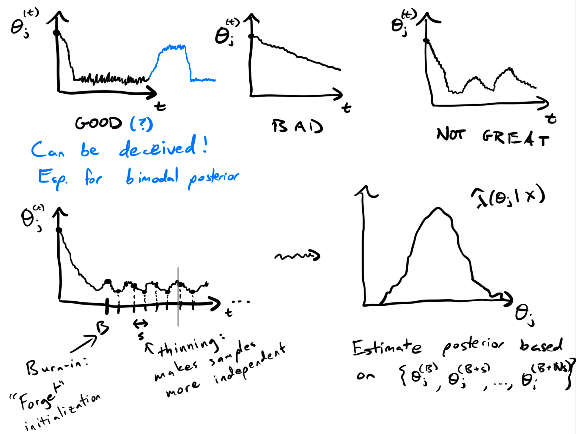
3 MCMC in Practice

• In theory, pick any initialization ${\displaystyle {\theta }^{(0)}}$ and valid kernel ${\displaystyle Q}$, sample long enough s.t. ${\displaystyle {\theta }^{(t)}\sim \lambda (\theta |X)}$.
  Do it again ${\displaystyle N}$ more times, we have ${\displaystyle N}$ samples from ${\displaystyle \lambda (\theta |X)}$.
• In practice, we need to determine if we've sampled long enough.

For the last (desirable) one, the posterior mean is $$\frac{1}{N+1}\sum _{k=0}^N{\theta }_j^{B+ks}\to \mathbb{E}[{\theta }_j|X].$$

But this will cause Gibbs to take a long time to mix. (The image is a very sharp ellipse.) A better parameterization is $$\{\begin{array}{rl}& {\beta }_1={\theta }_1+{\theta }_2,\\ & {\beta }_2={\theta }_1-{\theta }_2,\end{array}$$ so ${\displaystyle {\beta }_1\perp \perp {\beta }_2|X}$. The Gibbs sampler is equivalent to directly sampling from posterior.

4 Empirical Bayes

Back to the Gaussian hierarchical model $$\frac{1}{d}||X|{|}^2\sim \frac{1+{\tau }^2}{d}{\chi }_d^2\sim (1+{\tau }^2,\frac{2(1+{\tau }^2)}{d}),$$ the MLE for ${\displaystyle 1+{\tau }^2}$ is ${\displaystyle \frac{1}{d}||X|{|}^2}$.
For any "reasonable" prior, ${\displaystyle \mathbb{E}[\zeta |X]\approx \frac{d}{||X|{|}^2}}$, which should be close to MLE. $${\hat{\theta }}_i\approx (1-\frac{d}{||X|{|}^2})\approx (1-\zeta )X_i.$$

If prior doesn't matter much, why use one? Could just estimate ${\displaystyle \zeta }$ from data however we want, "plug it in".

UMVUE: ${\displaystyle \hat{\zeta }=\frac{d-2}{||X|{|}^2}}$.

Call Empirical Bayes a hybrid approach in which hyperparameters are treated as fixed, others treated as random.